- Published on
The Essentials - Graph Fundamentals & Traversal Methods
- Authors

- Name
- Abhishek Goudar
A 10-Minute Read
- I. Introduction: The Universal Language of Graphs
- II. Graph Fundamentals: Defining the Components
- Definitions
- Critical Graph Properties
- III. Data Structures for Graphs: Representation Analysis
- IV. Depth-First Search (DFS): Vertical Exploration
- V. Breadth-First Search (BFS): Layered Exploration
- Conclusion
I. Introduction: The Universal Language of Graphs
Graph theory stands as a pivotal field within discrete mathematics and computer science, offering a foundational mathematical structure for modeling complex pairwise relationships between objects. Graphs are the essential language used to map everything from logistical networks and biological interactions to the sprawling architectures of social media platforms and the interconnected web itself. Understanding the mechanics of how these structures are represented and explored is non-negotiable for practitioners operating in advanced computing environments.
The utility of a graph lies in its ability to encode connectivity. However, this structure is inert without efficient mechanisms to explore its components. Graph traversal algorithms, specifically Depth-First Search (DFS) and Breadth-First Search (BFS), are the primary tools developed for systematically analyzing these connections. These algorithms are not merely abstract concepts; they are fundamental building blocks required for sophisticated operations such as determining reachability, finding shortest paths, generating topological orderings, and identifying connected components in real-world systems. Mastering these traversals, along with their underlying data structures and complexity constraints, forms the core competency for graph-based problem-solving.
II. Graph Fundamentals: Defining the Components
A rigorous discussion of graph algorithms necessitates precise terminology regarding the components and properties of the graph structure itself.
Of course. Here is the updated text, which now directly references the different plots in the image you provided to illustrate each concept.
Definitions

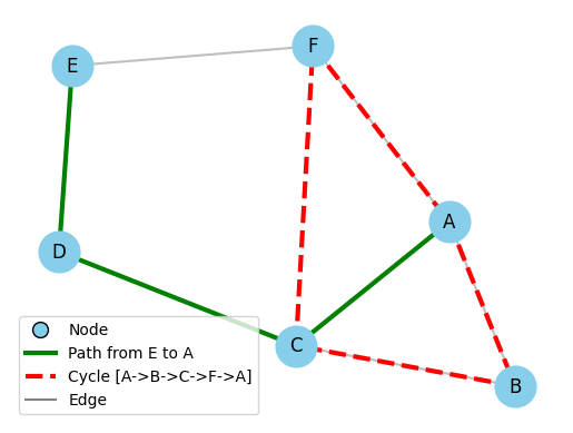
1. Node (Vertex, ) The node, or vertex, is the fundamental entity within a graph. Nodes represent the objects being related, such as cities in a map or users in a network. In Figure 1, the labeled circles (A, B, C, etc.) are the nodes. The total count of nodes is represented by .
2. Edge (Link, ) An edge represents the connection or relationship between two vertices. In the visualizations, these are the lines connecting the nodes. The gray lines in Figure 1 represent edges. The total count of edges is represented by .
3. Path A path is a sequence of distinct vertices connected by edges. The green solid line in Figure 1 highlights a specific path from node E to node A.
4. Cycle A cycle is a path that initiates and terminates at the same vertex. The red dashed line in Figure 1 illustrates a cycle, which starts at node A and returns after passing through B, C, and F.
Critical Graph Properties
1. Directed vs. Undirected

The directionality of edges defines the nature of the relationship.
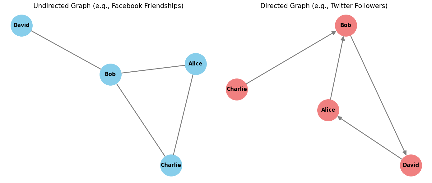
Undirected Graphs: Edges represent a symmetric relationship (). If A is connected to B, B is connected to A. As shown in the "Undirected Graph (Friendships)" in Figure 2, a simple line between "Alice" and "Bob" signifies a mutual friendship.
Directed Graphs (Digraphs): Edges are directional, representing an asymmetric relationship (). A connection from A to B does not imply a connection from B to A. The "Directed Graph (Followers)" in Figure 2 illustrates this with an arrow: "Alice" follows "Bob", but the reverse is not guaranteed. Traversal is restricted to the direction of the edges.
2. Weighted vs. Unweighted

This distinction is crucial, as it dictates the selection of appropriate pathfinding algorithms.
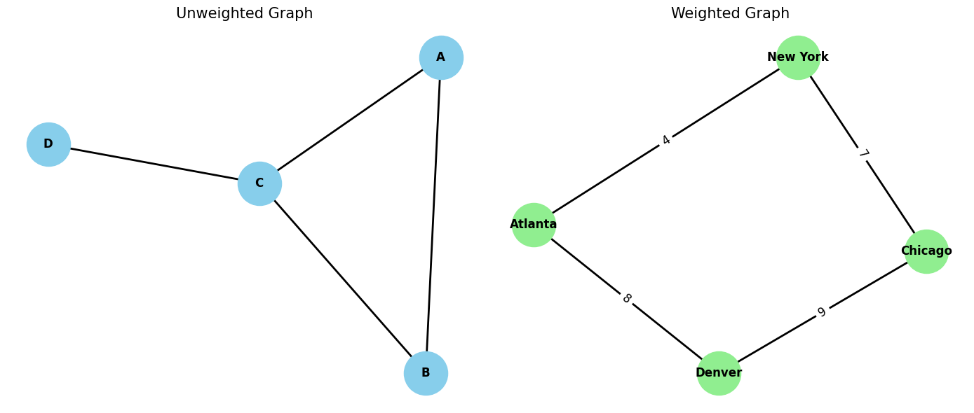
Weighted Graphs: Each edge has an associated numerical value, or weight. The "Weighted Graph" in Figure 3 demonstrates this by showing numbers on each edge, which could represent distance or cost between cities. The length of a path is the sum of these weights.
Unweighted Graphs: Edges simply indicate connectivity. The "Unweighted Graph" in Figure 3 shows this clearly, with no numerical values on its edges. Here, the shortest path is the one with the fewest "hops" or edges.
The selection of a representation (weighted or unweighted) has profound algorithmic consequences. While standard Breadth-First Search (BFS) is optimal for finding the shortest path in terms of the number of edges in an unweighted graph, it fails to find the true least-cost path in a weighted graph. For problems where edge weights are meaningful, more complex shortest-path algorithms, such as Dijkstra’s or , must be employed.
III. Data Structures for Graphs: Representation Analysis
The efficiency of any graph algorithm hinges critically upon the underlying data structure chosen to represent the graph. Two primary methods exist: the Adjacency Matrix and the Adjacency List.

Adjacency Matrix Representation
An Adjacency Matrix is a square matrix, let's call it , where is the number of vertices. Each entry in the matrix encodes the relationship between vertex and vertex .
- For a weighted graph, the entry stores the weight of the edge connecting vertex and vertex . If no edge exists, the value is 0.
- For an unweighted graph, if an edge exists, and otherwise.
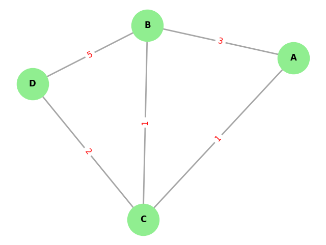
The matrix below represents the weighted graph from Figure 4. Notice that the diagonal entries are all zero, which signifies that there are no self-loops (i.e., no edges connecting a vertex to itself). For an undirected graph like this one, the matrix is symmetric ().
The primary advantage of the Adjacency Matrix is its speed in checking for the existence of an edge between any two given vertices , which is an operation. However, its space complexity is a fixed , regardless of the number of edges. This makes it suitable primarily for dense graphs, where the number of edges () is close to .
Adjacency List Representation (The Standard)
The Adjacency List is the industry-standard representation for graphs, particularly for the sparse graphs common in real-world applications. It consists of an array or hash map where each index or key corresponds to a vertex. The value associated with each vertex is a list of its adjacent neighbors.
For a weighted graph, this list stores pairs (or tuples) containing both the neighbor's identifier and the weight of the connecting edge. For the graph in Figure 4, the Adjacency List would be:
This structure is highly preferred because its space complexity is . Since it only stores data for existing edges, it is extremely space-efficient for sparse graphs, where .
Comparative Analysis of Graph Representations
The choice between matrix and list is usually driven by the graph's density and the required operational performance. The following table contrasts the complexities of various fundamental operations:
| Operation/Complexity | Adjacency Matrix | Adjacency List | Significance |
|---|---|---|---|
| Space Complexity | List is highly space-efficient for sparse graphs. | ||
| Edge Lookup | , or avg. | Matrix offers superior constant-time lookup. | |
| Adding a Vertex | List is far superior for dynamic/growing graphs. | ||
| Adding an Edge | Both perform equally well. | ||
| Removing an Edge | Matrix is faster as it requires no list search. |
The comparative analysis reveals a clear pattern favoring the Adjacency List for dynamic systems. While the matrix offers constant-time edge lookups and removals, the rigid cost associated with adding or removing a vertex in an Adjacency Matrix is prohibitive for graphs that evolve over time (such as social networks or routing tables). Conversely, the Adjacency List allows a new vertex to be added in time, confirming its status as the superior standard for efficient traversal algorithms.
IV. Depth-First Search (DFS): Vertical Exploration
Depth-First Search (DFS) is a traversal algorithm that explores as far as possible along each branch before backtracking. It operates on a "deep before wide" principle, systematically following a path until it reaches a terminal node or a previously visited one.
The core of DFS is its reliance on backtracking. When a path is exhausted, the algorithm returns to the most recent junction with unexplored paths and continues its deep dive from there. This Last-In, First-Out (LIFO) behavior is naturally implemented using a Stack (either explicitly in an iterative approach or implicitly via the call stack in recursion). Its depth-seeking nature makes it highly effective for tasks like cycle detection, pathfinding, and topological sorting.
The Role of the Stack
DFS relies exclusively on the Stack data structure to manage the state of traversal and implement the necessary backtracking mechanism.
- Recursive Implementation: The system's implicit Call Stack acts as the LIFO structure. When the recursion hits a base case (a dead end), the function returns, popping its state off the call stack and automatically achieving the required backtracking.
- Iterative Implementation: An explicit Stack is used. The node popped from the top of the stack is the next node processed, ensuring that the most recently added node's path is explored first.
Detailed Step-by-Step Walk-Through
The algorithm requires a Stack () and a Visited set () to track visited nodes and manage backtracking.
Initialization:
- Create an empty Stack ().
- Create an empty Visited set ().
- Add the source node () to .
- Add the source node () to (mark as visited).
Loop: Continue the process while is not empty.
Process:
- Pop the top element of .
- Process (e.g., print it or analyze it).
Explore Neighbors: Examine all adjacent vertices of .
- Condition Check: For each neighbor , check if is not in .
- Stacking: If has not been visited:
- Add to (mark as visited).
- Push onto .
Termination: The traversal concludes when the stack is empty, signifying all reachable paths have been exhausted.
Implementation (Python Code)
The following examples use an Adjacency List structure implemented as a Python dictionary.
DFS Iterative Implementation
def dfs_recursive(graph, node, visited):
    if node not in visited:
        print(node, end=' ')
        visited.add(node)
        # Recurse for each neighbor
        for neighbour in graph.get(node, []):
            dfs_recursive(graph, neighbour, visited)

# Example usage (same graph as iterative for consistency):
graph_example = {
    'A': ['B', 'C', 'D'],
    'B': ['E'],
    'C': ['G', 'F'],
    'D': ['H'],
    'E': ['I'],
    'F': ['J'],
    'G': ['K'],
    'H': [],
    'I': [],
    'J': [],
    'K': []
}
visited_set = set()
print("DFS traversal using recursive approach:")
dfs_recursive(graph_example, 'A', visited_set)
# Output: A B E I C G K F J D H
DFS Recursive Implementation
def dfs_iterative(graph, start):
    visited = set()
    stack = [start]

    while stack:
        node = stack.pop() # LIFO operation

        if node not in visited:
            print(node, end=' ')
            visited.add(node)

            # Add neighbors in reverse order to ensure proper depth-first sequence
            stack.extend(reversed(graph.get(node, [])))

# Example usage (same graph):
graph_example = {
    'A': ['B', 'C', 'D'],
    'B': ['E'],
    'C': ['G', 'F'],
    'D': ['H'],
    'E': ['I'],
    'F': ['J'],
    'G': ['K'],
    'H': [],
    'I': [],
    'J': [],
    'K': []
}
print("\nDFS traversal using iterative approach:")
dfs_iterative(graph_example, 'A')
# Output: A B E I C G K F J D H (consistent with recursion for this order)
V. Breadth-First Search (BFS): Layered Exploration
Breadth-First Search (BFS) is a traversal algorithm that explores a graph layer by layer, operating on a "wide before deep" principle. It systematically visits all neighbors at the current distance (or "level") from the source node before advancing to nodes at the next level.
This level-by-level exploration is managed by a Queue, which follows a First-In, First-Out ( FIFO) principle. The most significant application of BFS is its ability to find the shortest path in unweighted graphs. Because it discovers nodes in increasing order of their distance (number of edges) from the source, the first time it reaches a target node, it is guaranteed to be via the shortest possible path.
The Role of the Queue
BFS relies exclusively on the Queue data structure, which adheres to a First-In, First-Out (FIFO) principle. The queue ensures that nodes are processed in the order they were discovered, thus guaranteeing that all nodes at a current level are fully processed before the algorithm begins exploring the next level.
Detailed Step-by-Step Walk-Through
The algorithm requires a Queue () and a Visited set () to prevent cycles and redundant work.
Initialization:
- Create an empty Queue ().
- Create an empty Visited set ().
- Add the source node () to .
- Add the source node () to (mark as visited).
Loop: Continue the process while is not empty.
Process:
- Dequeue the front element of .
- Process (e.g., print it, record its distance, or analyze it).
Explore Neighbors: Examine all adjacent vertices of .
- Condition Check: For each neighbor , check if is not in (i.e., it has not been visited).
- Enqueuing: If has not been visited:
- Add to (mark as visited).
- Enqueue into .
Termination: The process repeats until the queue is empty, indicating all reachable vertices have been visited.
Implementation (Python Code)
The standard BFS implementation uses the deque class from Python's collections module for efficient queue operations.
BFS Iterative
from collections import deque

def bfs(graph, start):
    """
    Perform Breadth-First Search (BFS) on a graph starting from a given node.

    Parameters:
    graph (dict): Adjacency list representation of the graph.
    start: The starting vertex.

    Returns:
    list: A list of vertices in the order they were visited.
    """

    visited = set()           # To keep track of visited nodes
    queue = deque([start])    # Initialize queue with the starting node
    order = []                # To store the traversal order

    while queue:
        vertex = queue.popleft()   # Dequeue the front element
        if vertex not in visited:
            visited.add(vertex)    # Mark as visited
            order.append(vertex)   # Record the visit

            # Enqueue all unvisited neighbors
            for neighbor in graph.get(vertex, []):
                if neighbor not in visited:
                    queue.append(neighbor)

    return order


# Example usage:
if __name__ == "__main__":
    # Example graph represented as an adjacency list
    graph = {
        'A': ['B', 'C'],
        'B': ['D', 'E'],
        'C': ['F'],
        'D': [],
        'E': ['F'],
        'F': []
    }

    traversal = bfs(graph, 'A')
    print("BFS Traversal Order:", traversal)
BFS Recursive
from collections import deque
from collections import deque
def bfs_recursive(graph, queue, visited, order):
    if not queue:
        return

    vertex = queue.popleft()
    if vertex not in visited:
        visited.add(vertex)
        order.append(vertex)

        for neighbor in graph.get(vertex, []):
            if neighbor not in visited:
                queue.append(neighbor)

    bfs_recursive(graph, queue, visited, order)

# Example usage:
if __name__ == "__main__":
    graph_recursive = {
        'A': ['B', 'C'],
        'B': ['D', 'E'],
        'C': ['F'],
        'D': [],
        'E': ['F'],
        'F': []
    }
    visited = set()
    queue = deque(['A'])
    order = []
    bfs_recursive(graph_recursive, queue, visited, order)

    print("BFS Recursive Traversal Order:", order)
Conclusion
By now, you should have a solid understanding of graph structures, the trade-offs between the Adjacency Matrix and the efficient Adjacency List ( space), and the mechanics of the two cornerstone traversal algorithms.
- DFS () uses a stack to prioritize depth, making it ideal for checking connectivity and finding cycles.
- BFS () uses a queue to explore breadth-first, guaranteeing the shortest path in unweighted graphs.
Mastering these fundamental concepts is the crucial first step toward tackling advanced topics like Dijkstra's algorithm, Topological Sort, and maximum flow problems. Graphs are the backbone of modern data science and computer engineering. Keep traversing! 🗺️